Traffic Control Systems Handbook: Chapter 3. Control Concepts - Urban And Suburban Streets

Page 1

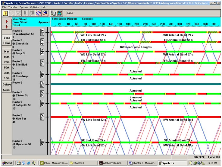
Figure 3-1. Time-Space Diagram Display from Synchro 4.

3.1 Introduction

This chapter discusses traffic control concepts for urban and suburban streets. In planning and designing a traffic signal control system, one must first understand the applicable operational concepts related to signalized intersection control and signal-related special control.

Signalized intersection control concepts include:

• Isolated intersection control - controls traffic without considering adjacent signalized intersections.
• Interchange and closely spaced intersection control - provides progressive traffic flow through two closely spaced intersections, such as interchanges. Control is typically done with a single traffic controller.
• Arterial intersection control (open network) - provides progressive traffic flow along the arterial. This is accomplished by coordination of the traffic signals.
• Closed network control - coordinates a group of adjacent signalized intersections.
• Areawide system control - treats all or a major portion of signals in a city (or metropolitan area) as a total system. Isolated, open- or closed-network concepts may control individual signals within this area.

Signal-related special control concepts include:

• High occupancy vehicle (HOV) priority systems.
• Preemption - Signal preemption for emergency vehicles, railroads, and drawbridges.
• Priority Systems - Traffic signal control strategies that assign priority for the movement of transit vehicles.
• Directional controls - Special controls designed to permit unbalanced lane flow on surface streets and changeable lane controls.
• Television monitoring.
• Overheight vehicle control systems.

A number of commonly used proprietary traffic systems and simulations are discussed in this chapter. These discussions provide illustrations of the technology and are not intended as recommendations. As these and similar products continue to be improved, the reader is advised to contact the supplier for the latest capabilities of these products.

3.2 Control Variables

Control variables measure, or estimate, certain characteristic of the traffic conditions. They are used to select and evaluate on-line control strategies and to provide data for the off-line timing of traffic signals. Control variables commonly used for street control include:

• Vehicle presence,
• Flow rate (volume),
• Occupancy and density,
• Speed,
• Headway, and
• Queue length.

Generally, presence detectors (refer to Chapter 6) sense these traffic variables. Table 3-1 describes the verbal and mathematical definition of these variables.

Table 3-1. Control Variable Definitions

Variable	Definition	Equation
Vehicle Presence	Presence (or absence) of a vehicle at a point on the roadway	N/A
Flow Rate	Number of vehicles passing a point on the roadway during a specified time period	Q = Vehicles/hour passing over detector N = Number of vehicles counted by detector during time period, T T = Specified time period, in hours
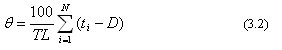
Occupancy	Percent of time that a point on the roadway is occupied by a vehicle	Where: = Raw occupancy, in percent T = Specified time period, in seconds L = Ratio of the effective length of the vehicle plus the loop to the vehicle length ti = Measured detector pulse presence, in seconds N = Number of vehicles detected in the time period, TD = Detector drop out time – detector pickup time
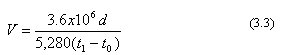
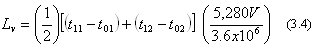
Speed	Distance traveled by a vehicle per unit time	Either one or two detectors can measure speed (see Figure 3-2). Where: One Detector (passage time) V = Speed, in mi/hr d = Mean vehicle length plus effective loop length, in ft t0 = Time when detector turns on, in millisec(ms) t1 = Time when detector turns off, in ms Two Detector (speed trap) d = Distance between detectors, in ft t0 = Time upstream detectors turns on, in ms t1 = Time downstream detector turnson, in ms Traffic control systems commonly use this equation, which assumes a vehicle moves at constant velocity through the two-detector speed trap. Speed traps are more commonly used for freeway surveillance. 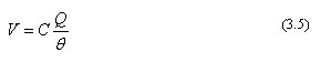The vehicle length, Lv, in ft may be determined from a speed-trap measurement as follows: Where: V = Speed determined from the speed-trap calculation, in mi/hr t0i = Time when ith detector of speed-trap turns on, in milliseconds t1i = Time when ith detector of speed-trap turns off, in milliseconds For the first detector i = 1, for the second detector i = 2. An alternative method shown in equation 3.5 can compute the average speed over a cycle T from volume and occupancy (1) Where C is a calibration coefficient best obtained experimentally
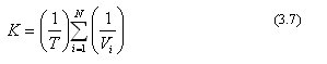
Density	Number of vehicles per lane mi (km)	Where: Q = Volume of traffic flow, in v/hr K = Density of traffic flow, in v/mi Üs= Space-mean speed, in mi/hr While density is an important quantity in traffic flow theory, most traffic control systems do not use this parameter directly for implementing flow control. Density (K) may be directly computed from count and speed measurements by equation 3.7. Where: N = The number of vehicles detected during time, T Vi = Speed of vehicle i crossing a detector in a lane K = Density of detectorized lane
Headway	Time spacing between front of successive vehicles, usually in one lane of a roadway	Time difference between beginning of successive vehicle detections (see Figure 3-3)
Queue Length	Number of vehicles stopped in a lane behind the stopline at a traffic signal	N/A

In addition, certain environmental factors influence traffic performance. Environmental conditions include:

• Pavement surface conditions (wet or icy),
• Weather conditions (rain, snow or fog).

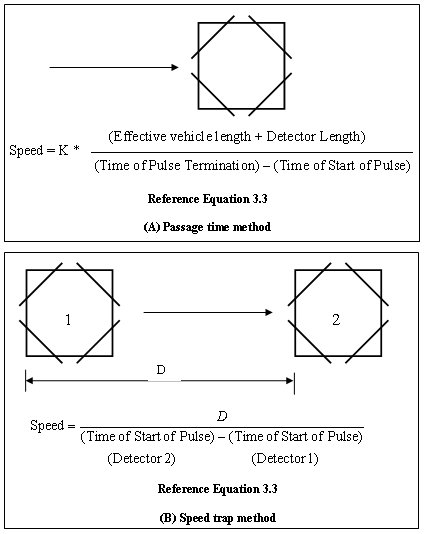
Figure 3-2. Speed Measurements Using Presence Detectors.

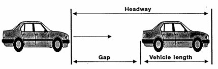
Figure 3-3. Headway determination.

3.3 Sampling

A microprocessor at the field site usually samples presence detectors to establish the detector state, thus replicating the detector pulse. The finite time between samples generates an error in the pulse duration that leads to errors in speed (most noticeable) and occupancy.

Equation 3.8 represents the maximum percentage error for any vehicle:

Where:

%E = Percent error in occupancy
S = Inverse of the sampling rate, seconds per sample
T = Presence time for a vehicle with an average length at a given speed.

Based on its statistical distribution, the standard deviation of the percentage error becomes:

Averaging data over a period of time reduces this error. Most modern traffic control systems provide a sufficiently small value of S so that the sampling error is negligible.

3.4 Filtering and Smoothing

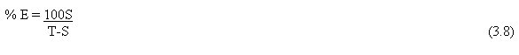
Traffic data, may be viewed as consisting of two distinct components, nonrandom and random. These components are described in Table 3-2 (2).

Table 3-2. Traffic Data Components

Component	Characteristic	Source
Nonrandom	Deterministic	Changes in basic service demand Ability of intersection to service demand
Random	Varies about deterministic component Characterized by a Poisson or other probability distribution	Nondeterministic changes in value from cycle to cycle

Figure 3-4 (a) shows a typical 30-minute sample of detector volume data obtained during a period when the deterministic component remained essentially constant. Figure 3-4 (b) shows the occupancy data for that period during which the signal system operated with a 1-minute cycle and without smoothing (to be discussed later). Thus, the volumes represent actual counts sensed by the detector.

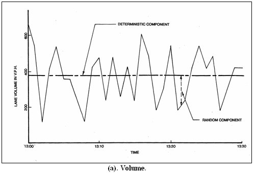
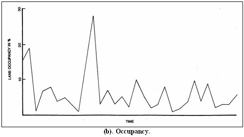
Figure 3-4. Deterministic and Random Components When Demand Is Constant

Figure 3-5 shows a typical example of a deterministic component representing an A.M. peak period condition (2). In many conventional traffic control systems, the traffic-responsive control law should respond quickly and accurately to the deterministic data components. Because both the deterministic and random components appear together in the detector data, this objective can only be accomplished imperfectly. A first order data filter often provides data smoothing to suppress the random component. The smoothing equation that performs this function is:

Where:

= Filter output after the mth computation
x(m) = Filter input data value (average value of variable between m-1 and m instants)
K = Filter coefficient in the range 0 to 1.0; (K=1 represents no filtering)

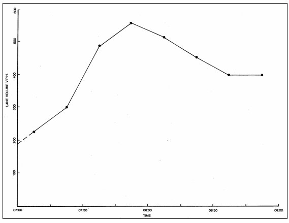
Figure 3-5. Deterministic Component of Volume during A.M. Peak Period.

Figure 3-6 shows the smoothing effect of the filter on the traffic data of Figure 3-4 (a) when processed by Equation 3.10 with various values for K (2).

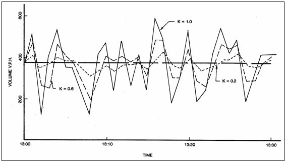
Figure 3-6. Effect Of Variation In Smoothing Coefficient On Random Component

Although the filter reduces the effect of the random component, it develops an error in the faithful reproduction of the deterministic component when that component is changing.

Figure 3-7 (a) shows the lag in the filter output. Figure 3-7 (b) shows the magnitude of this error for the input data of Figure 3-5.

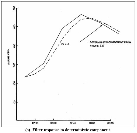
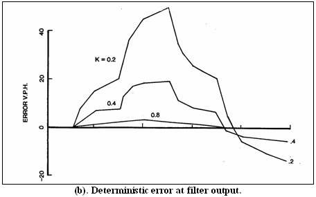
Figure 3-7. Filter Response And Output To Deterministic Component And Error

Gordon describes a technique for identifying the appropriate coefficient by determining the coefficient which equates the errors developed by both components (2).

3.5 Traffic Signal Timing Parameters

Table 3-3 provides definitions of the fundamental signal timing variables.

Table 3-3. Signal Timing Variable Definitions

Variable	Definition
Cycle Length	The time required for one complete sequence of signal intervals (phases).
Phase	The portion of a signal cycle allocated to any single combination of one or more traffic movements simultaneously receiving the right-of-way during one or more intervals.
Interval	A discrete portion of the signal cycle during which the signal indications (pedestrian or vehicle) remain unchanged.
Split	The percentage of a cycle length allocated to each of the various phases in a signal cycle.
Offset	The time relationship, expressed in seconds or percent of cycle length, determined by the difference between a defined point in the coordinated green and a system reference point.

3.6 Traffic Signal Phasing

Phasing reduces conflicts between traffic movements at signalized intersections. A phase may involve:

• One or more vehicular movements,
• One or more pedestrian crossing movements, or
• A combination of vehicular and pedestrian movements.

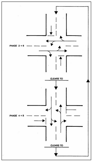
The National Electrical Manufacturers Association (NEMA) has adopted and published precise nomenclature for defining the various signal phases to eliminate misunderstanding between manufacturers and purchasers (95). Figure 3-8 illustrates the assignment of right-of-way to phases by NEMA phase numbering standards and the common graphic techniques for representing phase movements. In this figure, the signal cycle consists of 2 primary phase combinations (Phases 2 + 6 and Phases 4 + 8), which provide partial conflict elimination. This arrangement separates major crossing movements, but allows left-turn movements to conflict. This may prove acceptable if left-turn movements remain light; but if heavy, these movements may also require separation. Figure 3-9 illustrates a 4-phase sequence separating all vehicular conflicts. Section 7.7 more fully discusses the NEMA phase designations.

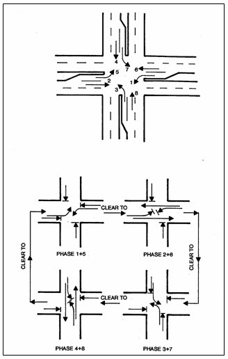Figure 3-8. Two-phase Signal Sequence	Figure 3-9. Four-phase Signal Sequence

Phasing Options

Left-Turn Phasing

As suggested by the previous discussion, phasing becomes primarily a left-turn issue. As left-turns and opposing through volumes increase, the engineer should consider left-turn phasing. Figure 3-10 identifies left-turn phasing options.

The most common practice allows opposing left-turns to move simultaneously as concurrently timed phases.

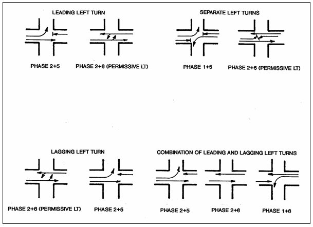
Figure 3-10. Dual-Ring Left-Turn Phasing Options.

Holding the number of phases to a minimum generally improves operations. As the number of phases increases, cycle lengths and delays generally increase to provide sufficient green time to each phase. The goals of improving safety (by adding left-turn phases) and operations at a signalized intersection may conflict, particularly with pretimed control.

Table 3-4 shows advantages and disadvantages of other options for left-turn phasing.

Table 3-4. Additional Left-turn Phasing Options

Option	Advantage	Disadvantage
Use traffic actuated instead of pretimed left-turn phase	Gives unused left-turn phase time to related through traffic movement	Requires additional detectors
Provide protected / permissive left-turn movement	Reduces delay and queuing	High speeds, blind or multilane approaches or other circumstances may preclude this technique
Change left-turn phase sequences with timing plan changes	Improves progression	Motorists may not expect changed phase sequences

Although the Manual on Uniform Traffic Control Devices (MUTCD) (3) does not provide warrants for left-turn phasing, several States and local agencies have developed their own guidelines. The Manual of Traffic Signal Design and the Traffic Control Devices Handbook summarize representative examples of these guidelines (4, 5).

Reference 6 provides a set of guidelines for left-turn protection. The report provides guidance on:

• Justification of protected left-turn phasing,
• Type of left-turn protection, and
• Sequencing of left-turns.

Phase Sequencing

Operational efficiency at a signalized intersection, whether isolated or coordinated, depends largely on signal phasing versatility. Variable-sequence phasing or skip-phase capability proves particularly important to multiphase intersections where the number of change intervals and start-up delay associated with each phase can reduce efficiency considerably. Each set of stored timing plans has a distinct phase sequence.

Full-actuated traffic control illustrates variable-sequence phasing. In the upper part of Figure 3-11, all approach lanes have detectors. Using these detectors, actuated control skips phases with no traffic present and terminates certain movements when their traffic moves into the intersection. This capability produces a variation in the phasing sequence. The lower part of Figure 3-11 illustrates primary phasing options for a full-actuated intersection. The phasing options selected may be changed with the signal timing plan.

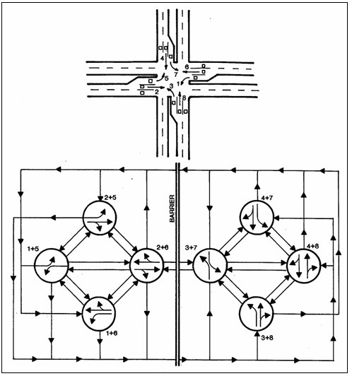
Figure 3-11. Primary Phasing Options For 8-Phase Dual-Ring Control (Left-Turn First).

3.7 Isolated Intersections

The major considerations in the operation of an isolated intersection are:

• Safe and orderly traffic movement,
• Vehicle delay, and
• Intersection capacity.

Vehicle delay results from:

• Stopped time delay (time waiting during red), and
• Total delay (stopped time delay plus stop and start-up delay).

Ideally, the objectives of minimizing total delay will:

• Maximize intersection capacity, and
• Reduce the potential for accident-producing conflicts.

However, these two objectives may not prove compatible. For example, using as few phases as possible and the shortest practical cycle length lessens delay. However, reducing accidents may require multiple phases and longer cycles, as well as placement of approach detectors to eliminate effects of a possible dilemma zone (see section 6.3). This placement may not be the optimum choice to reduce delays. Therefore, it is necessary to apply sound engineering judgment to achieve the best possible compromise among these objectives.

Traffic Flow

Flow characteristics of traffic are fundamental in analyzing intersection delay or capacity. Vehicles occupy space and, for safety, require space between them. With vehicles moving continuously in a single lane, the number of vehicles passing a given point over time will depend on the average headway. For example, for an average headway of 2 seconds, a volume of 1800 v/hr (3600 sec/hr x 1 v/2 sec) results.

Two factors influence capacity at a signalized intersection:

• Conflicts occur when two vehicles attempt to occupy the same space at the same time. This requires allocation of right-of-way to one line of vehicles while the other line waits.
• The interruption of flow for the assignment of right-of-way introduces additional delay. Vehicles slow down to stop and are also delayed when again permitted to proceed.

These factors (interruption of flow, stopping, and starting delay) reduce capacity and increase delay at a signalized intersection as compared to free-flow operations. Vehicles that arrive during a red interval must stop and wait for a green indication and then start and proceed through the intersection. The delay as vehicles start moving is followed by a period of relatively constant flow.

Table 3-5 presents data on typical vehicle headways (time spacing) at a signalized intersection as reported by Greenshields (7). These data illustrate basic concepts of intersection delay and capacity.

Table 3-5. Vehicle Headway Data

Position in Line	Observed Time Spacing (Sec)	Time Spacing at Constant Flow (Sec)	Added Startup Time (Sec)
1	3.8	2.1	1.7
2	3.1	2.1	1
3	2.7	2.1	0.6
4	2.4	2.1	0.3
5	2.2	2.1	0.1
6 and over	2.1	2.1	0
Source: Reference 7

Types of Control

Traffic signal control for isolated intersections falls into two basic categories:

• Pretimed, and
• Semi- and fully traffic actuated.

Each type offers varying performance and cost characteristics depending on the installation and prevailing traffic conditions.

Chang (8) provides guidelines and information to aid the engineer in selecting the appropriate type of signal control as shown in Figure 3-12. As shown in Tables 3-6 and 3-7, Skabardonis (17) also provides guidelines. Figure 3-13 shows possible arrangements for inductive loop detectors for actuated approaches and Figure 3-14 shows an example of actuated phase design.

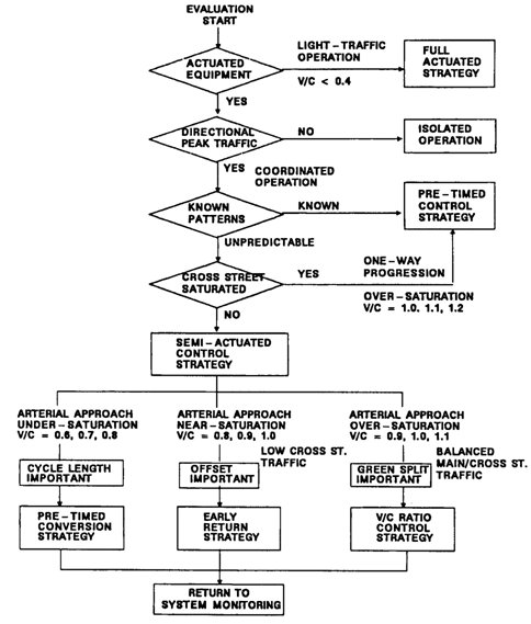
Figure 3-12. Recommended Selection Guidelines

Table 3-6. Proposed Signal Control at Specific Intersections Along Arterials

Cross Street Traffic V/C	Turning Movements*	Arterial Volume/Cross Street Volume
		< 1.3	> 1.3
Low to Moderate V/C < 0.8	< 20 Percent	Actuated (1)	Actuated (2)
	> 20 Percent	Actuated (2)	Actuated
High V/C > 0.8	< 20 Percent	Pretimed	Pretimed
	> 20 Percent	Pretimed	Pretimed
*Percent of arterial through traffic. Notes: · Pretimed control at intersection with balanced volumes and high turning traffic from the cross street without exclusive lanes. · Pretimed operation if the early start of the green leads to additional stops and delay at the downstream signal. Also, boundary intersections may operate as pretimed if they are critical to the arterial's time-space diagram and define the leading edge of the green bandwidth.

Table 3-7. Proposed Signal Control at Specific Intersections in Grid Systems

Network Configuration	Intersection V/C	Number of Phases
		2	4	8
Crossing Arterials	< 0.80 Percent	Pretimed	Actuated (1)	Actuated (1)
	> 0.80 Percent	Pretimed	Pretimed (2)	Pretimed (2)
Dense Network	< 0.80 Percent	Fully Actuated (3)	Actuated	Fully Actuated
	> 0.80 Percent	Pretimed	Actuated	Fully Actuated
Notes: · The through phases may operate as pretimed if the volumes on each arterial are approximately equal, or semi-actuated operated leads to additional stops at the downstream signal(s). · Left turn phases at critical intersections may operate as actuated. Any spare green time from the actuated phases can be used by the through phases. · Intersections that require a much lower cycle than the system cycle length and are located at the edge of the network where the progression would not be influenced.

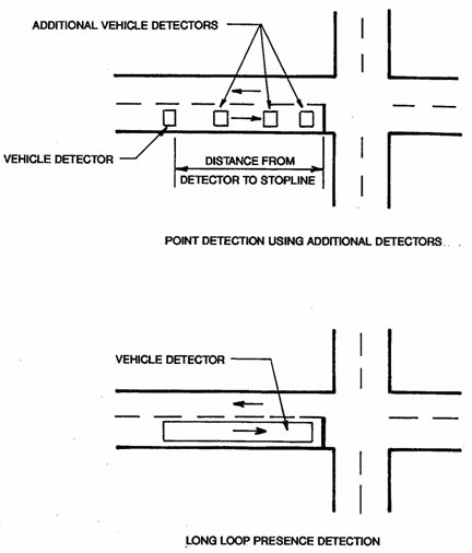
Figure 3-13. Traffic Detection On Intersection Approach

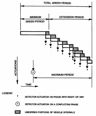
Figure 3-14. Example of Actuated Phase Intervals.

Intersection Timing Requirements

Pretimed Controller

For pretimed control at isolated intersections, the engineer must determine:

• Cycle length,
• Phase lengths or cycle split (green interval plus yellow change interval), and
• Number and sequence of phases.

Traffic-Actuated Control

Traffic detectors on an actuated approach working in conjunction with timing values for each of the phases (see Table 3-8) determine the phase length.

Table 3-8. Interval Settings

Interval	Requirement	Calculation/Operation
Minimum Green	Basic (no Volume-Density Feature): Service number of cars potentially stored between detector and stopline or the number normally stopped if a single detector is located a significant distance from the stopline Remains constant	Point detection: Compute minimum green interval times for various detector setback distances assuming: Start-up delay of 4 seconds Average headway between discharging vehicles of 2 seconds Minimum green time at least (4 + 2 N), where N is number of vehicles between detector and stopline Compute N assuming an average vehicle length of 26 ft (7.9 m). For detectors located approximately 120 ft (36.6 m) or more from the stopline, minimum green may equal 14 seconds or longer. The length of minimum green time reduces ability to respond to traffic demand changes. Therefore, consider 120 ft (36.6 m) as upper limit for single detector placement and at speeds of 35 mi/hr (56.3 km/hr) or less. Where pedestrians cross and no separate pedestrian crossing indications exist, (e.g., WALK-DON'T WALK), minimum green time should ensure adequate pedestrian crossing time. Long loop presence detection (or a series of short loops): Set initial interval close to zero when the detector loop ends at the stopline. If the loop ends at some distance from the stopline, use this distance to determine initial interval with point detection. See Chapter 6 for further discussion of vehicle detector placement and relationship to approach speed.
	Traffic-Actuated (Volume-Density Feature): Initial interval based on number of vehicle actuations stored while other phases serviced	When there are serviceable calls on opposing phases, and no additional vehicles cross the detector, terminate phase at the end of this minimum green time. Where pedestrians cross and no separate pedestrian crossing indications exist, (e.g., WALK-DON'T WALK), minimum green time should ensure adequate pedestrian crossing time.
Passage Time (Vehicle interval, extension interval, or unit extension)	Time required by a vehicle to travel from detector to intersection. With a call waiting on an opposing phase, represents the maximum time gap between vehicle actuations that can occur without losing the green indication. As long as the time between vehicle actuations remains shorter than the vehicle interval (or a present minimum gap), green will be retained on that phase subject to maximum interval.	Once the passage time interval timing is initiated and an additional vehicle is detected, present vehicle interval timing is canceled and a new vehicle interval timing initiated. This process is repeated for each additional vehicle detection until: Gap-out occurs (the gap between detections is greater than the vehicle interval or a present minimum gap). Max-out occurs (the interval timing reaches a preset maximum and a pedestrian or a vehicle call has been placed for another phase). In either of these two cases, the timing of a yellow change interval is initiated and the phase terminated. If the vehicle interval is not completely timed out (because of the maximum override), then a recall situation is set and the timing will return to this phase at the first opportunity. Figure 3-14 illistrates the situation where: Successive actuations occurred. Gaps shorter than passage time interval. Preset maximum green interval reached. Long loop presence detection: Set passage time interval close to zero because the signal controller continuously extends the green as long as loop is occupied. In this case, critical time gap is time required for a vehicle to travel a distance equal to the loop length plus the vehicle length. For a series of short loops, treat them as a long loop, provided that the distance between loops is less than the vehicle length; otherwise, use a short vehicle interval to produce the equivalent effect of a single long loop.
Maximum Green (Total green time or vehicle extension limit)	Maximum length of time a phase can hold green in presence of conflicting call.	Reference 9 provides detailed guidance.

Timing Considerations

Cycle Length and Split Settings

HCM 2000 (10) provides a detailed description of computational procedures for cycle and split settings. The following discussion summarizes some of the key items in the HCM.

Figure 3-15 depicts the traffic signal cycle, and Figure 3-16 provides definitions for this figure. Equation 3.11 provides an estimate of lost time (t_L for each signal phase). A value of 4 seconds is suggested unless local measurements provide a more accurate value.

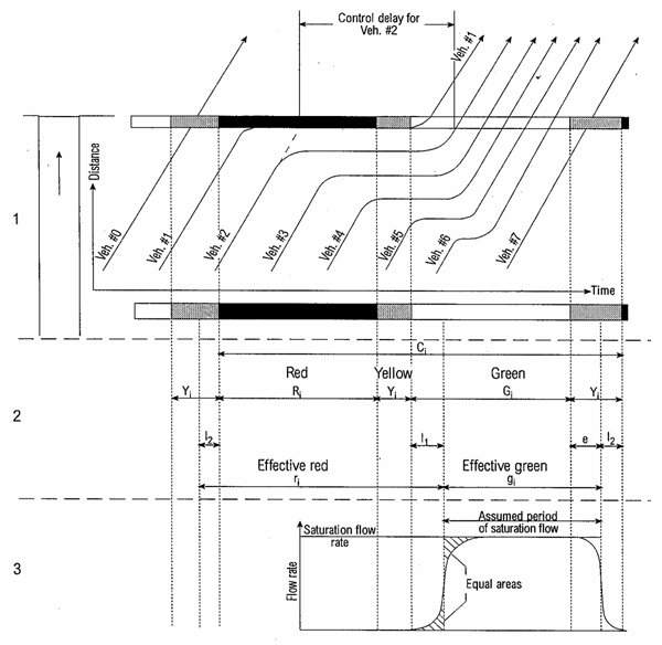
Figure 3-15. Fundamental Attributes of Flow at Signalized Intersections.

Name	Symbol	Definition	Unit
Change and clearance interval	Yi	The yellow plus all-red interval that occurs between phases of a traffic signal to provide for clearance of the intersection before conflicting movements are released	S
Clearance lost time	l2	The time between signal phases during which an intersection is not used by any traffic	S
Control delay	di	The component of delay that results when a control signal causes a lane group to reduce sped or to stop; it is measured by comparison with the uncontrolled condition	S
Cycle		A complete sequence of signal indications
Cycle length	Ci	The total time for a signal to complete one cycle length	S
Effective green time	gi	The time during which a given traffic movement or set of movements may proceed; it is equal to the cycle length minus the effective red time	S
Effective red time	ri	The time during which a given traffic movement or set of movements is directed to stop; it is equal to the cycle length minus the effective green time	S
Extension of effective green time	e	The amount of the change and clearance interval, at the end of the phase for a lane group, that is usable for movement of its vehicles	S
Green time	Gi	The duration of the green indication for a given movement at a signalized intersection	S
Interval		A period of time in which all traffic signal indications remain constant
Lost time	tL	The time during which an intersection is not used effectively by any movement; it is the sum of clearance lost time plus start-up lost time	S
Phase		The part of the signal cycle allocated to any combination of traffic movements receiving the right-of-way simultaneously during one or more intervals
Red time	Ri	The period in the signal cycle during which, for a given phase or lane group, the signal is red	S
Saturation flow rate	si	The equivalent hourly rate at which previously queued vehicles can traverse an intersection approach under prevailing conditions, assuming that the green signal is available at all times and no lost times are experienced	veh/h
Start-up lost time	l1	The additional time consumed by the first few vehicles in a queue at a signalized intersection above and beyond the saturation headway, because of the need to react to the initiation of the green phase and to accelerate	S
Total lost time	L	The total lost time per cycle during which the intersection is effectively not used by any movement, which occurs during the change and clearance intervals and at the beginning of most phases.	S

Figure 3-16. Symbols, Definitions, and Units for Fundamental Variables of Traffic Flow at Signalized Intersections.

Effective phase green time

HCM 2000 provides worksheets that facilitate the estimation of critical lane volume VCL.

Following the selection of a phasing plan, critical volumes (CV) are established for each phase. These are then used to calculate the cycle as follows.

A cycle length that will accommodate the observed flow rates with a degree of saturation of 1.0 is computed by Equation A10-1 in HCM 2000 and shown in equation 3.13 below. If the cycle length is known, that value should be used.

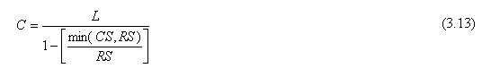
where:

C = cycle length (s),
L = total lost time (s),
CS = critical sum (veh/h), flow rate
RS = reference sum flow rate (1,710 * PHF * fa) (veh/h),
PHF = peak-hour factor, and
f_a = area type adjustment factor (0.90 if CBD, 1.00 otherwise).

RS is the reference sum of phase flow rates representing the theoretical maximum value that the intersection could accommodate at an infinite cycle length. The recommended value for the reference sum, RS, is computed as an adjusted saturation flow rate. The value of 1,710 is about 90 percent of the base saturation flow rate of 1,900 pc/h/ln. The objective is to produce a 90 percent v/c ratio for all critical movements.

The CS volume is the sum of the critical phase volume for each street. The critical phase volumes are identified in the quick estimation control delay and LOS worksheet on the basis of the phasing plan selected from Exhibit A10-8 in HCM 2000.

The cycle length determined from this equation should be checked against reasonable minimum and maximum values. The cycle length must not exceed a maximum allowable value set by the local jurisdiction (such as 150 s), and it must be long enough to serve pedestrians.

The ability to service traffic demand may be increased, up to a point, by increasing the cycle length. It is seen from Equation 3.13 that increasing the critical sum flow relative to the reference sum flow requires a higher cycle length to service the demand. Figure 3-17 shows the required cycle length for a two phase intersection (Lost time = 8 seconds).

The total cycle time is divided among the conflicting phases in the phase plan on the basis of the principle of equalizing the degree of saturation for the critical movements. The lost time per cycle must be subtracted from total cycle time to determine the effective green time per cycle, which must then be apportioned among all phases. This is based on the proportion of the critical phase flow rate sum for each phase determined in a previous step (10). The effective green time, g, (including change and clearance time) for each phase can be computed using Equation 3.14

Intersection Delay

The values derived from the delay calculations represent the average control delay experienced by all vehicles that arrive in the analysis period, including delays incurred beyond the analysis period when the lane group is oversaturated. Control delay includes movements at slower speeds and stops on intersection approaches as vehicles move up in queue position or slow down upstream of an intersection (10).

The average control delay per vehicle for a given lane group is given by Equation 15-1 in HCM 2000 as

where:

d = control delay per vehicle (s/veh);
d₁ = uniform control delay assuming uniform arrivals (s/veh);
PF = uniform delay progression adjustment factor, which accounts for effects of signal progression;
d₂ = incremental delay to account for effect of random arrivals and oversaturation queues, adjusted for duration of analysis period and type of signal control; this delay component assumes that there is no initial queue for lane group at start of analysis period (s/veh); and
d₃ = initial queue delay, which accounts for delay to all vehicles in analysis period due to initial queue at start of analysis period (s/veh)

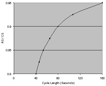
Figure 3-17. Cycle Length vs. Demand for Two Phase Signal.

Details for the estimation of d₁, PF, d₂ and d₃ are provided in HCM 2000.

Critical Lane Groups

HCM 2000 uses the concept of critical lane groups. A critical lane group is the lane group that has the highest flow ratio (ratio of volume to saturation flow) for the phase. The critical lane group determines the green time requirements for the phase.

Critical lane groups are used to identify a number of parameters in the signal timing process. One measure of the relative capacity of the intersection is the critical volume to capacity ratio for the intersection (X_C). It is given by:

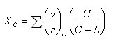
Where:

= summation of flow ratios for all critical lane groups i;
C = cycle length (s); and
L = total lost time per cycle, computed as lost time tL, for critical path of movement (s)

Traffic-Actuated Control

Using traffic-actuated control at isolated intersections enables the timing plan to continuously adjust in response to traffic demand. However, the potential to minimize delay and maximize capacity will only be realized with careful attention to:

• Type of equipment installed,
• Mode of operation,
• Location of detectors, and
• Timing settings.

Traffic-actuated control equipment automatically determines cycle length and phase lengths based on detection of traffic on the various approaches. The major requirement is to set the proper timing values for each of the functions provided by the controller unit (See Table 3-8).

Other Considerations

Methods are available for developing timing plans and are discussed in the following references:

• Traffic Engineering Handbook (11),
• Manual on Uniform Traffic Control Devices (3),
• Manual of Traffic Signal Design (4), and
• Traffic Engineering Theory and Practice (12).

In addition to cycle length and split calculations, the traffic engineer should consider several other important factors in developing timing plans for signal control.

Pedestrian movement often governs a timing plan. The engineer must provide sufficient green for pedestrians to cross the traveled way (see reference 11 for example). Where equipment permits, the pedestrian phase should be activated when the pedestrian- phase interval exceeds the vehicle interval. A number of publications (e.g. Reference 9) provide guidelines for timing pedestrian intervals.

Another important consideration is the length of the phase-change period. This period may consist of only a yellow change interval or may include an additional all-red clearance interval. The yellow interval warns traffic of an impending change in the right-of-way assignment. For a detailed discussion of these intervals refer to Reference 9.

In considering control concepts and strategies for isolated signalized intersections, the engineer must consider:

• Traffic flow fluctuations, and
• The random nature of vehicle and pedestrian arrivals.

The daily patterns of human activity influence traffic flow; it usually exhibits three weekday peak periods (A.M., midday, P.M.). Drew (13) has shown that even within a peak hour the 5-minute flow rates can prove as much as 15 to 20 percent higher than the average flow rate for the total peak hour period. He has further shown that a Poisson distribution best predicts vehicle arrivals for isolated intersections, indicating that considerable variation in arrival volume can occur on a cycle-to-cycle basis.

Proceed to Page 2 of Chapter 3 | Previous